Computing Combined Coverage Map with Custom RIS Parameters

This tutorial explains how to compute a combined coverage map, taking into account the contributions of both the transmitter and the placed RIS.

Note

Before executing this step, you must first compute and visualize the transmitter-only coverage map. Please follow the Computing Transmitter-Only Coverage Map tutorial beforehand.

1. Define RIS Target Points

   There are two ways to define the RIS target points:

   • Using the Target Points from Clustering:

     Note

     To use this option, you must first run the clustering algorithm to compute target points. Refer to the Finding RIS Target Points via K-means Clustering tutorial before proceeding.

     In the GUI, select the radio button “Use the target point(s) found via clustering algorithm”.

   • Manually Entering Target Point Coordinates:

     • Go to the labelframe “Manual trials” on the left side of the GUI.

     • Enter the number of RIS target points in the field “Number of target points”

     • Select the checkbox “Enter the target point(s) manually”.

     • A new input area will appear between the labelframe “Manual trials” and the labelframe “Optimization algorithm”.

     • Enter the x, y, z coordinates for each target point manually.

2. Enter RIS Parameters

   • Set the RIS center position under the labelframe “Enter RIS center position (m) (x,y,z)”.

   • Set the RIS height and width under “RIS height (m)” and “RIS width (m)”, respectively.

   Note

   To determine feasible RIS positions in the scene, refer to the Computing Feasible RIS Positions tutorial.

3. Choose Phase Profile Approach

   • Select the desired phase profile approach from the dropdown next to the textlabel “Choose phase profile approach”.

   • If “Manual entry” is selected:

     • A new menu appears near the menu with the labelframe “Select manual phase profile file (.json)”.

     • Click the “Browse” button to select the phase profile .json file.

4. Enable Amplitude Fluctuations (Optional)

   • In order to see the effect of amplitude fluctuations in each RIS tile, we can define uniform random RIS tile amplitude fluctuations, ranging from 0 to 1. To do that, check the checkbox “Enable uniform random RIS element amplitude fluctuations (range: [0.0, 1.0])”.

   • Enter the lower and upper bounds for amplitude fluctuations.

5. Computing combined coverage map

   • Press the button “Compute combined coverage map (TX + RIS)”.

   • After execution:

     • Combined coverage map with the contributions of the transmitter and the RIS (Fig. 1).

     • RIS coverage gain map showing the path gain improvement by placing the RIS (Fig. 2).

     • Cumulative distribution function (CDF) plot comparing the no-RIS case and all previous combined coverage cases (Fig. 3).

     • New binary poor coverage map after placing the RIS (Fig. 4).

   Additionally, the values for the new coverage ratio of the combined coverage map and the new average path gain of the low-power cells will be displayed under the labelframe “Messages”. If the operation ends without errors, the message “Combined coverage is analyzed successfully!” will appear.

An example scenario consisting of two RIS target points is shown below:

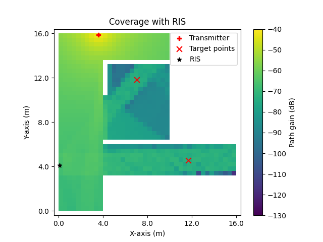
Fig. 1: Combined coverage map with the contributions of the transmitter and the RIS

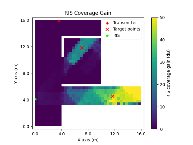
Fig. 2: RIS coverage gain map

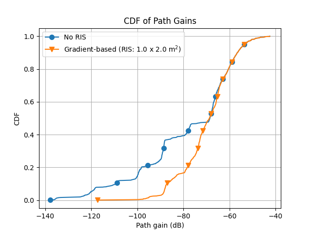
Fig. 3: Cumulative distribution function (CDF)

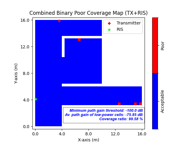
Fig. 4: New binary poor coverage map after placing the RIS