Computing Transmitter-Only Coverage Map
In this tutorial, the transmitter-only coverage map is computed and visualized for the previously specified scenario and other chosen parameters. You can choose to preset parameters using the “Preset parameters” button to fill all related parameters, including:
Scene frequency
TX position
Minimum path gain threshold
Coverage map cell size
However, before doing that, you need to load the predefined scenario under the labelframe “Scenario selection” by choosing the scenario from the list and pressing the “Load” button. If you wish to enter parameters manually, follow the instructions below:
Scenario Selection: A pre-defined scenario is selected from the list. Press the “Load” button under the labelframe “Scenario selection” in the GUI. If the scenario is successfully loaded, the message “Scene loaded successfully!” will appear in the bottom right under the labelframe “Messages”.
Scene Frequency: The communication frequency of the scene is specified in Hz under the labelframe “Scene frequency (Hz)”. For example, you can specify 5.8 GHz by typing “5.8e9”.
Transmitter (TX) Position: The transmitter coordinates (in meters) are entered under the labelframe “TX position (m) (x, y, z)”, starting with the x-coordinate as stated in the label.
Minimum Path Gain Threshold: This threshold defines the acceptable signal quality below which cells are considered low-power. You can type this value in dB under the labelframe “Minimum path gain threshold (dB)”. Please refer to our journal paper for more details.
Coverage Map Cell Size: The resolution of the coverage map can be defined by specifying the coverage map cell size (in meters) under the labelframe “Coverage map cell size (m)”. Be careful when defining this parameter since it depends on the predefined and loaded scenario. For example, if the scenario includes walls with a 0.4 m thickness, the coverage map cell size should be in ratio with that (e.g., 0.2 m or 0.4 m). A mismatch may result in incorrect interpretation of coverage map results due to the mixing of power levels inside the walls and non-wall areas.
Before computing the transmitter-only coverage map, you can preview the scenario using the “Preview scenario” button.
Once all the parameters are entered, press the “Compute TX-only coverage map” button. This may take some time depending on the resolution. After the computation, the following will be displayed:
Transmitter-only coverage map (Fig. 1)
Binary poor coverage map (Fig. 2), which shows the low-power cells in red (for further details, see our journal paper).
Additionally, the values for the coverage ratio of the TX-only coverage map and the average path gain of the low-power cells will be displayed under the labelframe “Messages”. If the operation ends without errors, the message “TX-only coverage map and binary poor coverage map plotted successfully!” will appear.
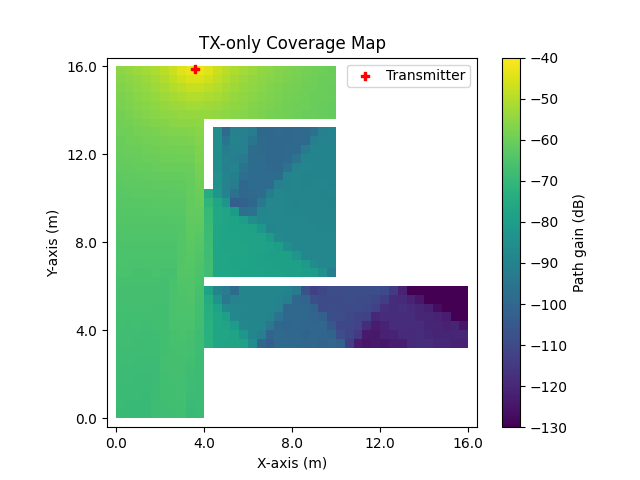
Fig. 1: Transmitter-only coverage map
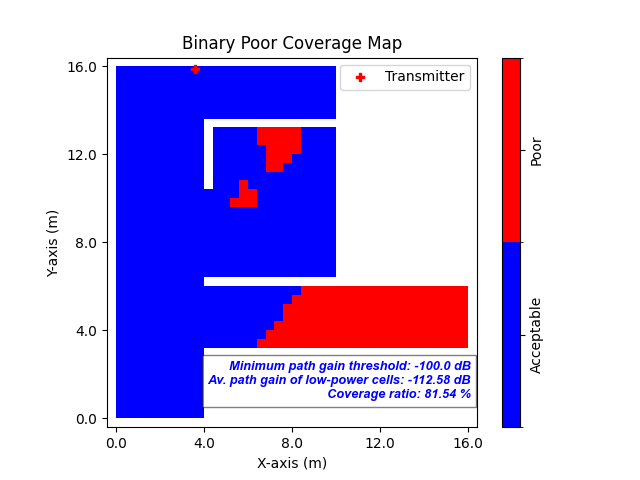
Fig. 2: Binary poor coverage map