Phase Error Performance Sensitivity Analysis
This tutorial explains how to analyze the sensitivity of performance when phase errors are introduced to the RIS elements within a specified delta range.
Simulation Procedure
In this analysis, the following steps are followed:
Ideal Phase Profile Calculation: The ideal phase profile for the RIS is computed for a given target configuration using the selected phase profile approach (e.g., Gradient-based, distance-based, or manual entry).
Introduction of Phase Errors: A uniform random phase error is added independently to each RIS element. The error for each element is sampled from a uniform distribution within \([-\Delta, +\Delta]\) radians:
\[\epsilon_{n,m} \sim \mathcal{U}(-\Delta, +\Delta)\]where \(\epsilon_{n,m}\) is the random phase error introduced to the \((n,m)\)-th RIS element, and \(\Delta\) is the maximum magnitude of the error (in radians, user-specified in degrees).
The resulting phase profile after introducing phase errors becomes:
\[\varphi_{n,m}^{\text{with error}} = \varphi_{n,m}^{\text{ideal}} + \epsilon_{n,m}\]where \(\varphi_{n,m}^{\text{ideal}}\) denotes the original (ideal) phase value.
Coverage Map Computation: Using the phase profile with errors, the coverage map is computed via a ray-tracing simulation.
Performance Metric Evaluation: The performance metric is evaluated as the average path gain of the predefined low-power cells.
Monte Carlo Averaging: Multiple realizations (random draws of phase errors) are performed for each delta value, and the average and standard deviation of the performance metric are computed across these realizations to obtain a statistically meaningful performance degradation curve.
Visualization: The average performance metric is plotted against the maximum phase error \(\Delta\) (in degrees), with error bars showing the standard deviation across realizations.
How to Perform Phase Error Sensitivity Analysis in the GUI
Note
Before executing this step, you must first compute and visualize the transmitter-only coverage map. Please follow the Computing Transmitter-Only Coverage Map tutorial beforehand.
Define RIS Target Points
There are two ways to define the RIS target points:
Using the Target Points from Clustering:
Note
To use this option, you must first run the clustering algorithm to compute target points. Refer to the Finding RIS Target Points via K-means Clustering tutorial before proceeding.
In the GUI, select the radio button “Use the target point(s) found via clustering algorithm”.
Manually Entering Target Point Coordinates:
Go to the labelframe “Manual trials” on the left side of the GUI.
Enter the number of RIS target points in the field “Number of target points”
Select the checkbox “Enter the target point(s) manually”.
A new input area will appear between the labelframe “Manual trials” and the labelframe “Optimization algorithm”.
Enter the x, y, z coordinates for each target point manually.
Enter RIS Parameters
Set the RIS center position under the labelframe “Enter RIS center position (m) (x,y,z)”.
Set the RIS height and width under “RIS height (m)” and “RIS width (m)”, respectively.
Note
To determine feasible RIS positions in the scene, refer to the Computing Feasible RIS Positions tutorial.
Conduct Sensitivity Analysis
Under the labelframe “Sensitivity analysis”, enter the minimum, maximum, and step values of \(\Delta\) (in degrees) to define the maximum phase error.
Specify the number of realizations to consider for each delta value. The final performance value is the average across all realizations.
Select which phase profile approaches (Gradient-based, distance-based, or manual) will be analyzed.
Press the button “Start sensitivity analysis” to initiate the procedure.
After execution, a figure will be generated showing the average performance metric versus \(\Delta\) (in degrees) for each selected approach, including error bars indicating standard deviation across random realizations. Two example figures are shown below for two different minimum path gain threshold considerations.
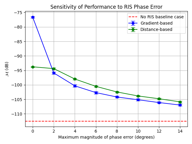
Fig. 1: Changes in performance metric \(\mathcal{M}\) (dB) vs. phase error magnitude \(\Delta\) (degrees) for different phase profile approaches with -100 dB minimum path gain threshold
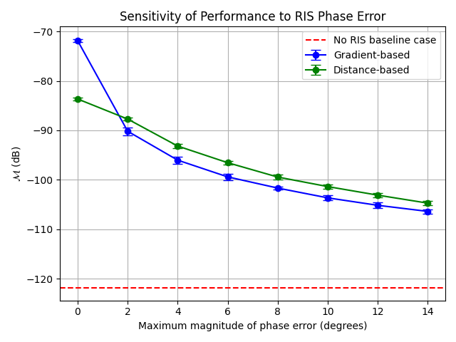
Fig. 1: Changes in performance metric \(\mathcal{M}\) (dB) vs. phase error magnitude \(\Delta\) (degrees) for different phase profile approaches with -110 dB minimum path gain threshold