Running RIS Joint Optimization Algorithm and Drawing Performance Evaluation Plots

This tutorial explains how to run the RIS joint optimization algorithm and how to draw performance evaluation plots after obtaining all performance metric results of all possible configurations.

Note

Before executing this step, you must first compute and visualize the transmitter-only coverage map. Please follow the Computing Transmitter-Only Coverage Map tutorial beforehand.

1. Choose Phase Profile Approach

   • Select the desired phase profile approach from the dropdown next to the textlabel “Choose phase profile approach”.

   • If “Manual entry” is selected:

     • A new menu appears near the menu with the labelframe “Select manual phase profile file (.json)”.

     • Click the “Browse” button to select the phase profile .json file.

2. Enter the Parameter Boundaries

   • Enter the lowest and highest number of target points, along with the step size for the search, under the labelframe “Number of target point interval (N_lower, N_upper, N_step)”, which is located under “Optimization algorithm”.

   • Enter the RIS height under “RIS height (m)”.

   • Enter the lowest and highest RIS widths, along with the step size for the search, under “RIS width interval (m) (W_RIS_lower, W_RIS_upper, W_RIS_step)”.

   • Choose a metric computation technique under the labelframe “Metric computation technique”:

     • If “Using coverage map” is chosen, the algorithm computes the full coverage map for each RIS configuration (more accurate but slower).

     • If “Using individual path computation” is chosen, the algorithm only computes the path gains at previously identified low-power cells (faster).

3. Compute performance metrics

   Click the button “Compute performance metrics for all N, W_RIS, r_RIS” to compute all performance metrics across all RIS configurations, including variations in the number of target points, RIS widths, and feasible RIS positions.

   Important

   This operation can take a considerable amount of time. Please do not close the program until the operation is completed or you see an error in the Python interpreter or under the labelframe “Messages”!

4. Draw Performance Metric vs. RIS Width and Show Sub-optimal RIS Parameters

   At the end of Step 3, all performance metric and coverage ratio results along with the corresponding RIS configurations will be automatically exported as a dictionary in a .json file in the root directory of the RIS optimization framework’s source code.

   To visualize the best configuration considering a performance improvement threshold:

   • Select the performance metric .json data file under the labelframe “Select performance metric file (.json)” by clicking the “Browse” button.

   • Select the coverage ratio .json data file under the labelframe “Select coverage ratio file (.json)” by clicking the “Browse” button.

   • Under the labelframe “Performance meric vs. RIS width and determine sub-optimal RIS parameters (N^opt, W_RIS^opt, r^opt)”, enter a performance improvement threshold (dB) value. This threshold defines the minimum performance gain required to justify increasing the RIS width.

   • Click the button “Plot performance metric vs. RIS width and determine sub-optimal RIS parameters” to visualize the results.

   An example of the resulting figure is shown below:

   

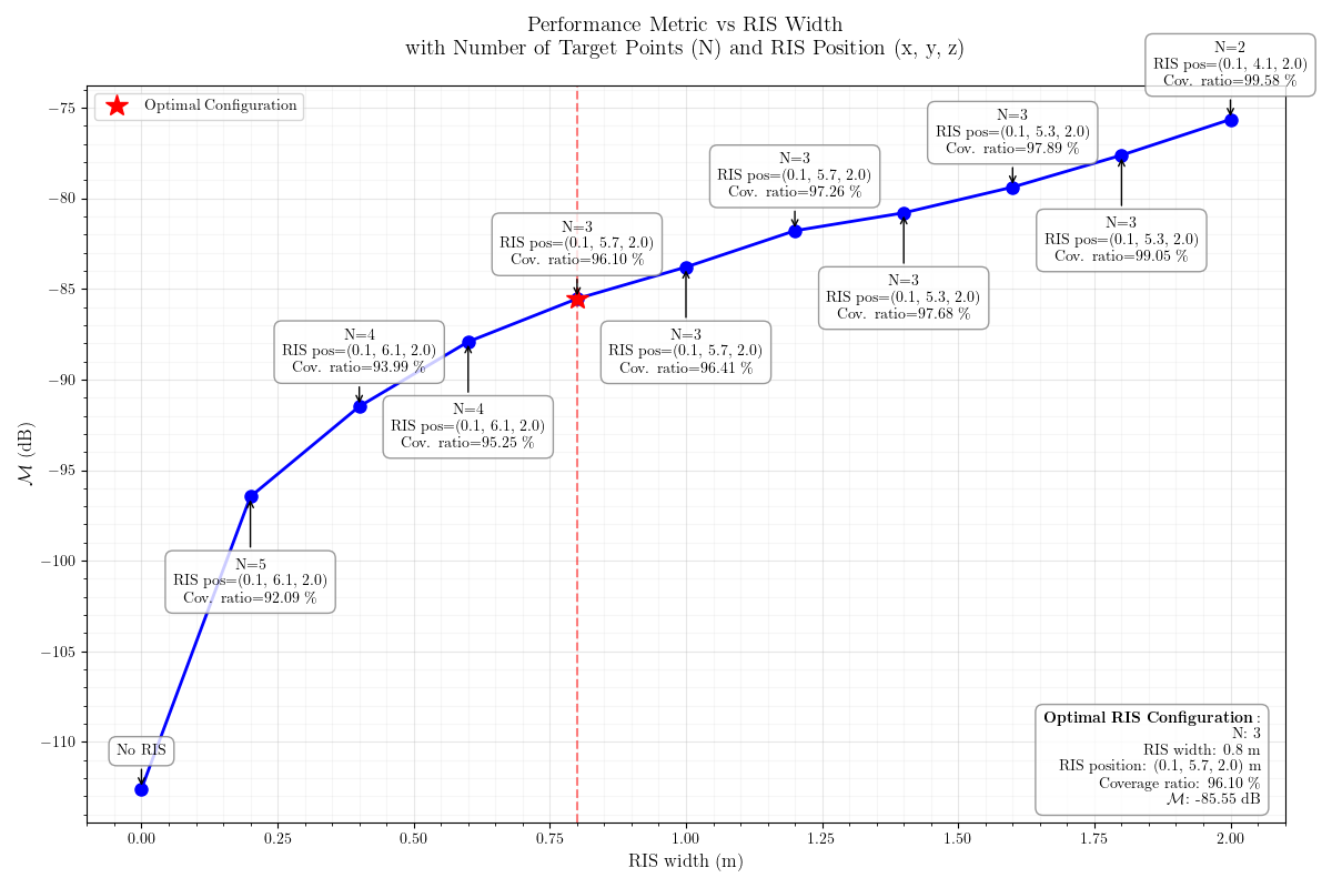
   Fig. 1: Performance metric vs. RIS width and sub-optimal RIS parameters

5. Draw Performance Metric vs. RIS Position

   As an alternative to Step 4, you can visualize the effect of RIS position on the selected performance metric.

   After computing all performance metrics in Step 3, proceed as follows:

   • Enter a RIS width value that is already present in the .json files.

     • The performance metric vs. RIS position plot will be generated for this specific RIS width.

     • The goal is to identify the best-performing configuration given the specified RIS width for each feasible RIS position.

     • A sub-optimal number of target points value (that yields the highest performance metric at each position) will also be shown as annotations on the plot.

   • Click the button “Plot performance metric vs. RIS position given the entered RIS width” to generate and display the plot.

   An example plot is shown below:

   

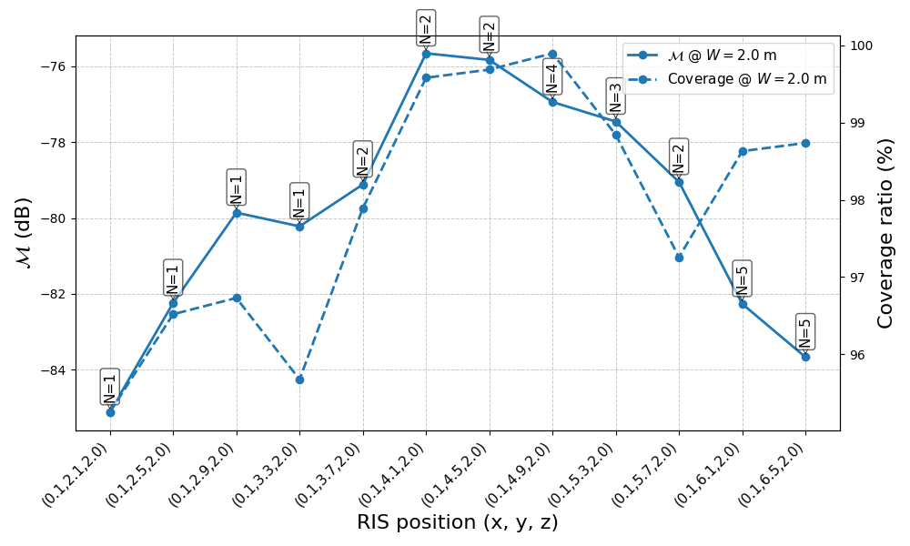
   Fig. 2: Performance metric vs. RIS position